stompy.spatial — Spatial analysis, data management and manipulation.

For GIS-related operations, and spatial tools to support model development and data analysis.

algorithms

General geometric algorithms that do not fit cleanly into more special-purpose modules.

stompy.spatial.algorithms.cut_polygon(poly, line)

field

Various classes representing a 2D scalar-valued function. Useful for bathymetry processing, creating parameter maps for model input. Includes both point-based and raster-based classes.

stompy.spatial.field.ApolloniusField

alias of stompy.spatial.field.PyApolloniusField

class stompy.spatial.field.BinopField(A, op, B)

Bases: stompy.spatial.field.Field

Combine arbitrary fields with binary operators

op2str()

str2op(s)

value(X)

in density_field this was called ‘scale’ - evaluates the field at the given point or vector of points. Some subclasses can be configured to interpolate in various ways, but by default should do something reasonable

class stompy.spatial.field.CompositeField(shp_fn=None, factory=None, priority_field='priority', data_mode='data_mode', alpha_mode='alpha_mode', shp_data=None, shp_query=None, target_date=None)

Bases: stompy.spatial.field.Field

In the same vein as BlenderField, but following the model of raster editors like Photoshop or the Gimp.

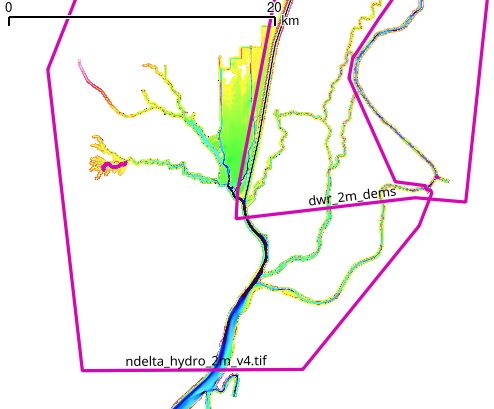
Individual sources are treated as an ordered “stack” of layers.

Layers higher on the stack can overwrite the data provided by layers lower on the stack.

A layer is typically defined by a raster data source and a polygon over which it is valid.

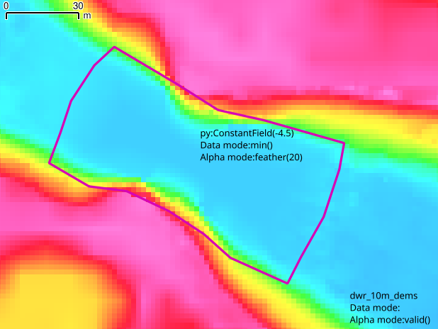
Each layer’s contribution to the final dataset is both a data value and an alpha value. This allows for blending/feathering between layers.

The default “data_mode” is simply overlay. Other data modes like “min” or “max” are possible.

The default “alpha_mode” is “valid()” which is essentially opaque where there’s valid data, and transparent where there isn’t. A second common option would probably be “feather(<distance>)”, which would take the valid areas of the layer, and feather <distance> in from the edges.

The sources, data_mode, alpha_mode details are taken from a shapefile.

Alternatively, if a factory is given, it should be callable and will take a single argument - a dict with the attributse for each source. The factory should then return the corresponding Field.

TODO: there are cases where the alpha is so small that roundoff can cause artifacts. Should push these cases to nan. TODO: currently holes must be filled manually or after the fact. Is there a clean way to handle that? Maybe a fill data mode?

Create a polygon shapefile, with fields:

priority	numeric
data_mode	string
alpha_mode	string

These names match the defaults to the constructor. Note that there is no reprojection support – the code assumes that the shapefile and all source data are already in the target projection. Some code also assumes that it is a square projection.

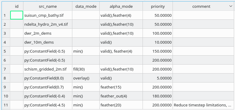
Each polygon in the shapefile refers to a source dataset and defines where that dataset will be used.

Datasets are processed as layers, building up from the lowest priority to the highest priority. Higher priority sources generally overwrite lower priority source, but that can be controlled by specifying data_mode. The default is overlay(), which simple overwrites the lower priority data. Other common modes are

• min(): use the minimum value between this source and lower priority data. This layer will only deepen areas.
• max(): use the maximum value between this source and lower priority data. This layer will only raise areas.
• fill(dist): fill in holes up to dist wide in this datasets before proceeding.

Multiple steps can be chained with commas, as in fill(5.0),min(), which would fill in holes smaller than 5 spatial units (e.g. m), and then take the minimum of this dataset and the existing data from previous (lower priority) layers.

Another example:

bounds()

load_source(i)

projection = None

to_grid(nx=None, ny=None, bounds=None, dx=None, dy=None, mask_poly=None)

render the layers to a SimpleGrid tile. nx,ny: number of pixels in respective dimensions bounds: xxyy bounding rectangle. dx,dy: size of pixels in respective dimensions. mask_poly: a shapely polygon. only points inside this polygon will be generated.

class stompy.spatial.field.ConstantField(c)

Bases: stompy.spatial.field.Field

value(X)

in density_field this was called ‘scale’ - evaluates the field at the given point or vector of points. Some subclasses can be configured to interpolate in various ways, but by default should do something reasonable

class stompy.spatial.field.ConstrainedScaleField(X, F, projection=None, from_file=None)

Bases: stompy.spatial.field.XYZField

Like XYZField, but when new values are inserted makes sure that neighboring nodes are not too large. If an inserted scale is too large it will be made smaller. If a small scale is inserted, it’s neighbors will be checked, and made smaller as necessary. These changes are propagated to neighbors of neighbors, etc.

As points are inserted, if a neighbor is far enough away, this will optionally insert new points along the edges connecting with that neighbor to limit the extent that the new point affects too large an area

add_point(pnt, value, allow_larger=False)

Insert a new point into the field, clearing any invalidated data and returning the index of the new point

check_all()

check_scale(i, old_value=None)

old_value: if specified, on each edge, if the neighbor is far enough away, insert a new node along the edge at the scale that it would have been if we hadn’t adjusted this node

r = 1.1

remove_invalid()

Remove nodes that are too big for their delaunay neighbors

safety_factor = 0.85

class stompy.spatial.field.CurvilinearGrid(X, F, projection=None)

Bases: stompy.spatial.field.QuadrilateralGrid

apply_xform(xform)

bounds()

plot(**kwds)

regrid(b, interpolation='nearest')

returns an F array corresponding to the field B interpolated onto our grid

xyz()

unravel to a linear sequence of points

class stompy.spatial.field.Field(projection=None)

Bases: object

Superclass for spatial fields

assign_projection(projection)

bounds()

bounds_in_cs(cs)

copy()

crop(rect)

envelope(eps=0.0001)

Return a rectangular shapely geometry the is the bounding box of this field.

make_xform(from_projection, to_projection)

projection()

quantize_space(quant)

reproject(from_projection=None, to_projection=None)

Reproject to a new coordinate system. If the input is structured, this will create a curvilinear grid, otherwise it creates an XYZ field.

to_grid(nx=None, ny=None, interp='linear', bounds=None, dx=None, dy=None, valuator='value')

bounds is a 2x2 [[minx,miny],[maxx,maxy]] array, and is required for BlenderFields bounds can also be a 4-element sequence, [xmin,xmax,ymin,ymax], for compatibility with matplotlib axis(), and Paving.default_clip.

specify one of:

nx,ny: specify number of samples in each dimension dx,dy: specify resolution in each dimension

interp used to default to nn, but that is no longer available in mpl, so now use linear.

value(X)

in density_field this was called ‘scale’ - evaluates the field at the given point or vector of points. Some subclasses can be configured to interpolate in various ways, but by default should do something reasonable

value_on_edge(e, samples=5, reducer=<function nanmean>)

Return the value averaged along an edge - the generic implementation just takes 5 samples evenly spaced along the line, using value()

xyz()

class stompy.spatial.field.Field3D(projection=None)

Bases: stompy.spatial.field.Field

class stompy.spatial.field.FunctionField(func)

Bases: stompy.spatial.field.Field

wraps an arbitrary function function must take one argument, X, which has shape […,2]

value(X)

in density_field this was called ‘scale’ - evaluates the field at the given point or vector of points. Some subclasses can be configured to interpolate in various ways, but by default should do something reasonable

class stompy.spatial.field.GdalGrid(filename, bounds=None, geo_bounds=None)

Bases: stompy.spatial.field.SimpleGrid

A specialization of SimpleGrid that can load single channel and RGB files via the GDAL library. Use this for loading GeoTIFFs, some GRIB files, and other formats supported by GDAL.

static metadata(filename)

Return the extents and resolution without loading the whole file

class stompy.spatial.field.GtxGrid(filename, is_vertcon=False, missing=9999, projection='WGS84')

Bases: stompy.spatial.field.SimpleGrid

class stompy.spatial.field.MultiRasterField(raster_file_patterns, **kwargs)

Bases: stompy.spatial.field.Field

Given a collection of raster files at various resolutions and with possibly overlapping extents, manage a field which picks from the highest resolution raster for any given point.

Assumes that any point of interest is covered by at least one field (though there may be slower support coming for some sort of nearest valid usage).

There is no blending for point queries! If two fields cover the same spot, the value taken from the higher resolution field will be returned.

Basic bilinear interpolation will be utilized for point queries.

Edge queries will resample the edge at the resolution of the highest datasource, and then proceed with those point queries

Cell/region queries will have to wait for another day

Some effort is made to keep only the most-recently used rasters in memory, since it is not feasible to load all rasters at one time. to this end, it is most efficient for successive queries to have some spatial locality.

bounds()

Aggregate bounds

build_index()

clip_max = inf

crop(rect=None)

dx

dy

error_on_null_input = 'any'

extract_tile(xxyy=None, res=None)

Create the requested tile from merging the sources. Resolution defaults to resolution of the highest resolution source that falls inside the requested region

max_count = 20

offset = 0.0

open_count = 0

order = 1

ordered_hits(xxyy)

prepare()

report()

Short text representation of the layers found and their resolutions

serial = 0

source(i)

LRU based cache of the datasets

to_grid(nx=None, ny=None, interp='linear', bounds=None, dx=None, dy=None, valuator='value')

Extract data in a grid. currently only nearest, no linear interpolation.

value(X)

X must be shaped (…,2)

value_on_edge(e, samples=None)

Subsample the edge, using an interval based on the highest resolution overlapping dataset. Average and return…

value_on_point(xy)

class stompy.spatial.field.PyApolloniusField(X=None, F=None, r=1.1, redundant_factor=None)

Bases: stompy.spatial.field.XYZField

Takes a set of vertices and the allowed scale at each, and extrapolates across the plane based on a uniform telescoping rate

static from_polylines(lines, values, r=1.1, redundant_factor=None)

insert(xy, f)

directly insert a point into the Apollonius graph structure note that this may be used to incrementally construct the graph, if the caller doesn’t care about the accounting related to the field - returns False if redundant checks are enabled and the point was deemed redundant.

interpolate(X)

static read_shps(shp_names, value_field='value', r=1.1, redundant_factor=None)

Read points or lines from a list of shapefiles, and construct an apollonius graph from the combined set of features. Lines will be downsampled at the scale of the line.

to_grid(*a, **k)

use the delaunay based griddata() to interpolate this field onto a rectilinear grid. In theory interp=’linear’ would give bilinear interpolation, but it tends to complain about grid spacing, so best to stick with the default ‘nn’ which gives natural neighbor interpolation and is willing to accept a wider variety of grids

Here we use a specialized implementation that passes the extent/stride array to interper, since lin_interper requires this.

interp=’qhull’: use scipy’s delaunay/qhull interface. this can additionally accept a radius which limits the output to triangles with a smaller circumradius.

value(X)

X must be shaped (…,2)

class stompy.spatial.field.QuadrilateralGrid(projection=None)

Bases: stompy.spatial.field.Field

Common code for grids that store data in a matrix

to_xyz()

class stompy.spatial.field.SimpleGrid(extents, F, projection=None)

Bases: stompy.spatial.field.QuadrilateralGrid

A spatial field stored as a regular cartesian grid. The spatial extent of the field is stored in self.extents (as xmin,xmax,ymin,ymax) and the data in the 2D array self.F

XY()

apply_xform(xform)

bounds()

contour(**kwds)

contourf(**kwds)

copy()

crop(rect=None, indexes=None)

default_interpolation = 'nearest'

delta()

downsample(factor, method='decimate')

method: ‘decimate’ just takes every nth sample

‘ma_mean’ takes the mean of n*n blocks, and is nan

and mask aware.

extract_tile(xxyy=None, res=None, match=None, interpolation='linear', missing=nan)

Create the requested tile xxyy: a 4-element sequence match: another field, assumed to be in the same projection, to match

pixel for pixel.

interpolation: ‘linear’,’quadratic’,’cubic’ will pass the corresponding order

to RectBivariateSpline.

‘bilinear’ will instead use simple bilinear interpolation, which has the added benefit of preserving nans.

missing: the value to be assigned to parts of the tile which are not covered by the source data.

fill_by_convolution(iterations=7, smoothing=0, kernel_size=3)

Better for filling in small seams - repeatedly applies a 3x3 average filter. On each iteration it can grow the existing data out by 2 pixels. Note that by default there is not a separate smoothing process - each iteration will smooth the pixels from previous iterations, but a pixel that is set on the last iteration won’t get any smoothing.

Set smoothing >0 to have extra iterations where the regions are not grown, but the averaging process is reapplied.

If iterations is ‘adaptive’, then iterate until there are no nans.

fill_by_griddata()

Basically griddata - limits the input points to the borders of areas missing data. Fills in everything within the convex hull of the valid input pixels.

gdalwarp = 'gdalwarp'

gradient()

compute 2-D gradient of the field, returning a pair of fields of the same size (one-sided differences are used at the boundaries, central elsewhere). returns fields: dFdx,dFdy

hillshade_scalar(azimuth_deg=225, zenith_deg=45, z_factor=10)

hillshade_shader(**kwargs)

int_nan = -9999

interpolate(X, interpolation=None, fallback=True)

interpolation can be nearest or linear

mask_outside(poly, value=nan, invert=False, straddle=None)

Set the values that fall outside the given polygon to the given value. Existing nan values are untouched.

Compared to polygon_mask, this is slow but allows more options on exactly how to test each pixel.

straddle: if None, then only test against the center point

if True: a pixel intersecting the poly, even if the center is not inside, is accepted. [future: False: reject straddlers]

plot(**kwds)

plot_hillshade(**kwds)

point_to_index(X)

polygon_mask(poly, crop=True, return_values=False)

similar to mask_outside, but: much faster due to outsourcing tests to GDAL returns a boolean array same size as self.F, with True for pixels inside the polygon.

crop: if True, optimize by cropping the source raster first. should provide identical results, but may not be identical due to roundoff.

return_vales: if True, rather than returning a bitmask the same size

as self.F, return just the values of F that fall inside poly. This can save space and time when just extracting a small set of values from large raster

static read(fname)

rect_to_indexes(xxyy)

shape

smooth_by_convolution(kernel_size=3, iterations=1)

Repeatedly apply a 3x3 average filter (or other size: kernel_size). Similar to the smoothing step of fill_by_convolution, except that the effect is applied everywhere, not just in the newly-filled areas.

to_curvilinear()

to_xyz()

The simple grid version is a bit smarter about missing values, and tries to avoid creating unnecessarily large intermediate arrays

trace_contour(vmin, vmax, union=True)

Trace a filled contour between vmin and vmax, returning a single shapely geometry (union=True) or a list of polygons (union=False). Uses matplotlib to do the actual contour construction.

Note that matplotlib is not infallible here, and complicated or large inputs can create erroneous output. gdal_contour might help.

upsample(factor=2)

value(X)

in density_field this was called ‘scale’ - evaluates the field at the given point or vector of points. Some subclasses can be configured to interpolate in various ways, but by default should do something reasonable

value_on_edge(e, samples=None, **kw)

Return the value averaged along an edge - the generic implementation just takes 5 samples evenly spaced along the line, using value()

warp(t_srs, s_srs=None, fn=None, extra='')

interface to gdalwarp t_srs: string giving the target projection s_srs: override current projection of the dataset, defaults to self._projection fn: if set, the result will retained, written to the given file. Otherwise

the transformation will use temporary files. opts: other

extra: other options to pass to gdalwarp

warp_to_match(target)

Given a separte field trg, warp this one to match pixel for pixel.

self and target should have meaningful projection().

write(fname)

write_gdal(output_file, nodata=None, overwrite=False)

Write a Geotiff of the field.

if nodata is specified, nan’s are replaced by this value, and try to tell gdal about it.

if output_file is “Memory”, will create an in-memory GDAL dataset and return it.

write_gdal_rgb(output_file, vmin=None, vmax=None)

xy()

xyz()

unravel to a linear sequence of points

class stompy.spatial.field.TileMaker(f, **kwargs)

Bases: object

Given a field, create gridded tiles of the field, including some options for blending, filling, cropping, etc.

dx = 2

dy = 2

filename_fmt = '%(left).0f-%(bottom).0f.tif'

fill_iterations = 10

force = False

merge()

output_dir = '.'

quantize = True

smoothing_iterations = 5

tile(xmin=None, ymin=None, xmax=None, ymax=None)

tx = 1000

ty = 1000

class stompy.spatial.field.XYZField(X, F, projection=None, from_file=None)

Bases: stompy.spatial.field.Field

add_point(pnt, value)

Insert a new point into the field, clearing any invalidated data and returning the index of the new point

apply_xform(xform)

bounds()

build_index(index_type=None)

clip_to_polygon(poly)

created_point(i)

crop(rect)

cs2cs(src='+proj=utm +zone=10 +datum=NAD27 +nadgrids=conus', dst='+proj=utm +zone=10 +datum=NAD83')

In place modification of coordinate system. Defaults to UTM NAD27 -> UTM NAD83

decimate(factor)

default_interpolation = 'linear'

delete_point(i)

deleted_point(i)

init_listeners()

interpolate(X, interpolation=None)

intersect(other, op, radius=0.1)

Create new pointset that has points that are in both fields, and combine the values with the given operator op(a,b)

inv_dist_interp(p, min_radius=None, min_n_closest=None, clip_min=-inf, clip_max=inf, default=None)

inverse-distance weighted interpolation This is a bit funky because it tries to be smart about interpolation both in dense and sparse areas.

min_radius: sample from at least this radius around p min_n_closest: sample from at least this many points

lin_interper(aspect=1.0)

listen(event, cb)

listener_count = 0

static merge(all_sources)

move_point(i, pnt)

nearest(p, count=1)

nn_interper(aspect=1.0)

outside_hull_fallback = True

plot(**kwds)

plot_on_boundary(**kwds)

plot_tri(**kwargs)

qhull_interper(max_radius=None)

static read(fname)

Read XYZField from a pickle file

static read_shp(shp_name, value_field='value')

rectify(dx=None, dy=None)

Convert XYZ back to SimpleGrid. Assumes that the data fall on a regular grid. if dx and dy are None, automatically find the grid spacing/extents.

to_grid(nx=2000, ny=2000, interp='linear', bounds=None, dx=None, dy=None, aspect=1.0, max_radius=None)

use the delaunay based griddata() to interpolate this field onto a rectilinear grid. In theory interp=’linear’ would give bilinear interpolation, but it tends to complain about grid spacing, so best to stick with the default ‘nn’ which gives natural neighbor interpolation and is willing to accept a wider variety of grids

Here we use a specialized implementation that passes the extent/stride array to interper, since lin_interper requires this.

interp=’qhull’: use scipy’s delaunay/qhull interface. this can additionally accept a radius which limits the output to triangles with a smaller circumradius.

to_xyz()

tri(aspect=1.0)

updated_point(i)

value(X)

X must be shaped (…,2)

within_r(p, r)

write(fname)

write_shp(shp_name, value_field='value')

write_text(fname, sep=' ')

class stompy.spatial.field.XYZText(fname, sep=None, projection=None)

Bases: stompy.spatial.field.XYZField

class stompy.spatial.field.ZLevelField(X, Z, F)

Bases: stompy.spatial.field.Field3D

One representation of a 3-D field. We have a set of XY points and a water column associated with each. Extrapolation pulls out the closest water column, and extends the lowest cell if necessary.

distance_along_transect()

extrapolate(x, y, z)

plot_surface()

plot_transect()

Plots the data in 2-D as if self.X is in order as a transect. The x axis will be distance between points. NB: if the data are not organized along a curve, this plot will make no sense!

shift_z(delta_z)

stompy.spatial.field.as_xxyy(p1p2)

stompy.spatial.field.random()

random_sample(size=None)

Return random floats in the half-open interval [0.0, 1.0).

Results are from the “continuous uniform” distribution over the stated interval. To sample \(Unif[a, b), b > a\) multiply the output of random_sample by (b-a) and add a:

(b - a) * random_sample() + a

size : int or tuple of ints, optional

Output shape. If the given shape is, e.g., (m, n, k), then m * n * k samples are drawn. Default is None, in which case a single value is returned.

out : float or ndarray of floats

Array of random floats of shape size (unless size=None, in which case a single float is returned).

>>> np.random.random_sample()
0.47108547995356098
>>> type(np.random.random_sample())
<type 'float'>
>>> np.random.random_sample((5,))
array([ 0.30220482,  0.86820401,  0.1654503 ,  0.11659149,  0.54323428])

Three-by-two array of random numbers from [-5, 0):

>>> 5 * np.random.random_sample((3, 2)) - 5
array([[-3.99149989, -0.52338984],
       [-2.99091858, -0.79479508],
       [-1.23204345, -1.75224494]])

stompy.spatial.field.with_plt(f)

gen_spatial_index

A generic interface to several implementations of spatial indexes.

stompy.spatial.gen_spatial_index.point_index_class_factory(implementation='best')

stompy.spatial.gen_spatial_index.rect_index_class_factory(implementation='rtree')

interp_4d module

A heat-diffusion method for interpolating sparse data in space and time onto a grid. This can be used to take point samples collected over time and create a spatially smooth interpolation which respects shorelines and other features in a computational grid.

interp_coverage

Special-purpose constrained linear interpolation. Used by some methods in field.

join_features

Join many line segments into topologically consistent rings or polygons (potentially with holes). Useful if you have a shoreline made of many line segments, but want a single shoreline polyline or polygon.

stompy.spatial.join_features.arc_to_close_line(points, n_arc_points=40)

Given a list of points, return an arc that closes the linestring, and faces away from the centroid of the points

stompy.spatial.join_features.clean_degenerate_rings(point_lists, degen_shpname='degenerate_rings.shp')

Given a list of lists of points - filter out point lists which represent degenerate rings, writing the invalid rings to a shapefile degen_shpname, and returning a list of only the valid rings. Unclosed linestrings are passed through.

set degen_shpname to None to disable that output.

stompy.spatial.join_features.find_exterior_ring(point_lists)

stompy.spatial.join_features.lines_to_polygons(new_features, close_arc=False, single_feature=True, force_orientation=True, return_open=False, min_area=0.0)

returns a list of Polygons and a list of features which were not part of a polygon force_orientation: ensure that interior rings have negative signed area return_open: if True, allow open linestrings, but they will be returned in a 3rd item. min_area: prune polygons with area below this threshold

stompy.spatial.join_features.lines_to_polygons_slow(new_features, close_arc=False, single_feature=True, force_orientation=True)

single_feature: False is not yet implemented! returns a list of Polygons and a list of features which were not part of a polygon force_orientation: ensure that interior rings have negative signed area

stompy.spatial.join_features.merge_lines(layer=None, segments=None)

Given an ogr LineString layer, merge linestrings by matching endpoints, and return a list of arrays of points.

if layer is given, it should be an ogr LineString layer if segments is given, it should be a list of numpy arrays, where each array is [N,2] giving points along a path.

this version only handles exact matches between endpoints

stompy.spatial.join_features.process_layer(orig_layer, output_name, tolerance=0.0, create_polygons=False, close_arc=False, single_feature=True, remove_duplicates=True)

remove_duplicates: if true, exactly duplicated nodes along a single path will be removed, i.e.

the linestring A-B-B-C will become A-B-C.

single_feature: only save the biggest feature

stompy.spatial.join_features.progress_message(str, steps_done=None, steps_total=None)

stompy.spatial.join_features.progress_printer(str, steps_done=None, steps_total=None)

stompy.spatial.join_features.tolerant_merge_lines(features, tolerance)

expects features to be formatted like the output of merge_lines, i.e. a list of numpy arrays

stompy.spatial.join_features.vector_mag(vectors)

vectors: xy vectors, shape […,2] return magnitude (L2 norm)

kdtree_spatialindex

Wrapper for using scipy’s kdtree as a spatial index.

class stompy.spatial.kdtree_spatialindex.RtreeKDTree(stream, interleaved=False)

Bases: object

wrap scipy KDTree spatial index to look as much like Rtree class as possible

delete(feat_id, rect)

feat_id_to_index(feat_id)

insert(feat_id, rect=None)

intersects(xxyy)

This should be made compatible with the regular RTree call…

nearest(rect, count)

refresh_tree()

linestring_utils

Simple methods for resampling a polyline to higher or lower resolution.

stompy.spatial.linestring_utils.as_density(d)

stompy.spatial.linestring_utils.distance_along(linestring)

stompy.spatial.linestring_utils.downsample_linearring(points, density, factor=None, closed_ring=1)

Makes sure that points aren’t too close together Allow them to be 0.3*density apart, but any edges shorter than that will lose one of their endpoints.

stompy.spatial.linestring_utils.left_normals(linestring)

For each point in the [N,2] linestring find the left-pointing unit normal vector, returned in a [N,2] array.

stompy.spatial.linestring_utils.resample_linearring(points, density, closed_ring=1, return_sources=False)

similar to upsample, but does not try to include the original points, and can handle a density that changes even within one segment of the input

stompy.spatial.linestring_utils.upsample_linearring(points, density, closed_ring=1, return_sources=False)

proj_utils

A few utility functions related to geographic projections, mainly the mapper() function.

Bundle up common projection operations

stompy.spatial.proj_utils.ll_to_utm(LL, center_lon=None)

stompy.spatial.proj_utils.mapper(src, dest)

use it like this:

m = mapper(“WGS84”,”EPSG:26910”) print m(array([-122,35]))

stompy.spatial.proj_utils.to_srs(s)

stompy.spatial.proj_utils.xform(src, dest)

qgis_spatialindex module

A wrapper for using the QGIS spatial index class in stompy.

class stompy.spatial.qgis_spatialindex.RtreeQgis(stream, interleaved=False)

Bases: object

wrap qgis internal spatial index to look as much like Rtree class as possible

delete(feat_id, rect)

insert(feat_id, rect=None)

intersects(xxyy)

This should be made compatible with the regular RTree call…

make_feature(feat_id, rect)

nearest(rect, count)

robust_predicates module

A pure python implementation of Jonathan Shewchuk’s robust geometric predicates. Exact evaluation of tests for collinearity (does point A fall left/right/on a line joining points B,C), and in-circle (does point D fall inside/outside/on a circle defined by points A,B,C).

stompy.spatial.robust_predicates.Absolute(a)

stompy.spatial.robust_predicates.Fast_Two_Sum(a, b)

stompy.spatial.robust_predicates.Split(a)

stompy.spatial.robust_predicates.Square(a)

stompy.spatial.robust_predicates.Two_Diff(a, b)

stompy.spatial.robust_predicates.Two_Diff_Tail(a, b, x)

stompy.spatial.robust_predicates.Two_One_Diff(a1, a0, b)

stompy.spatial.robust_predicates.Two_One_Sum(a1, a0, b)

stompy.spatial.robust_predicates.Two_Product(a, b)

stompy.spatial.robust_predicates.Two_Product_Presplit(a, b, bhi, blo)

stompy.spatial.robust_predicates.Two_Sum(a, b)

stompy.spatial.robust_predicates.Two_Two_Diff(a1, a0, b1, b0)

stompy.spatial.robust_predicates.Two_Two_Sum(a1, a0, b1, b0)

stompy.spatial.robust_predicates.counterclockwise(pa, pb, pc)

stompy.spatial.robust_predicates.counterclockwiseadapt(pa, pb, pc, detsum)

stompy.spatial.robust_predicates.estimate(e)

stompy.spatial.robust_predicates.fast_expansion_sum_zeroelim(e, f)

stompy.spatial.robust_predicates.incircle(pa, pb, pc, pd)

stompy.spatial.robust_predicates.incircleadapt(pa, pb, pc, pd, permanent)

stompy.spatial.robust_predicates.orientation(a, b, c)

maybe there are faster ways when all we care about is yes no, zero.

stompy.spatial.robust_predicates.scale_expansion_zeroelim(e, b)

wkb2shp module

Read and write data to/from shapefiles.

Functions for reading and writing shapefiles.

These are simple wrappers around OGR and Shapely libraries.

stompy.spatial.wkb2shp.shp2geom(shp_fn, use_wkt=False, target_srs=None, source_srs=None, return_srs=False, query=None, fold_to_lower=False)

Read a shapefile into memory as a numpy array. Data is returned as a record array, with geometry as a shapely geometry object in the ‘geom’ field.

target_srs: input suitable for osgeo.osr.SetFromUserInput(), or an existing osr.SpatialReference, to specify a projection to which the data should be projected. If this is specified but the shapefile does not specify a projection, and source_srs is not given, then an exception is raised. source_srs will override the projection in the shapefile if specified.

fold_to_lower: fold field names to lower case.

return_srs: return a tuple, second item being the text representation of the project, or

None if no projection information was found.

stompy.spatial.wkb2shp.wkb2shp(shp_name, input_wkbs, srs_text='EPSG:26910', field_gen=<function <lambda>>, fields=None, overwrite=False, geom_type=None, driver=None, layer_name=None)

Save data to a shapefile.

shp_name: filename.shp for writing the result or ‘MEMORY’ to return an in-memory ogr layer.

input_wkbs: list of shapely geometry objects for each feature. They must all

be the same geometry type (no mixing lines and polygons, etc.)

There are three ways of specifying fields:

field_gen: a function which will be called once for each feature, with

the geometry as its argument, and returns a dict of fields.

fields: a numpy structure array with named fields, or fields: a dict of field names, with each dictionary entry holding a sequence

of field values.

srs_text: sets the projection information when writing the shapefile. Expects a string, for example ‘EPSG:3095’ or ‘WGS84’.

driver: Directly specify an alternative driver, such as GPKG. if None, assumed

shapefile, unless shp_name is ‘memory’ in which case create an in-Memory layer. for GPKG, the optional layer_name argument can be used to name the layer which would default to the basename of the shp_name otherwise

Module contents